Will AI Repeat Electricity's Forty Years? What Three Industrial Revolutions Tell Us About Diffusion

science

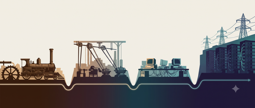
The clock of invention always runs faster than the clock of organisational change. Steam waited sixty years, the electric motor forty, the computer twenty. Today’s AI is standing at the start of the same curve.

1. A paradox that keeps recurring

In 1987 the economist Robert Solow made a remark that has been quoted ever since: “You can see the computer age everywhere but in the productivity statistics.”

That year the IBM PC had been on sale for six years and corporate IT spending was climbing annually — yet US productivity growth was slower than it had been before the 1970s. Only after 1995 did productivity visibly accelerate, twenty-five years after the microprocessor was born.

This is not peculiar to computers. Wind back a century: the electric motor had a commercial grid from 1882, but in 1899 motors accounted for only 5% of the mechanical power in American factories, and manufacturing productivity did not jump until the 1920s. Further back still, Watt received his patent for the separate condenser in 1769, but steam did not overtake water power until the 1830s — and steam’s peak contribution to British growth came roughly a century after Watt’s invention.

Every time a general-purpose technology appears, it goes through a long lag in which the technology already exists but the returns refuse to arrive. Sixty years, forty, twenty — the lag is shortening, but it has never gone to zero.

Understanding why that lag exists, and what determines its length, is the key to reading where today’s AI wave is going.

2. Steam: the technology existed for a century — why did nobody use it?

The story of the steam engine shows better than any other how far apart “the technology exists” and “the technology pays” can be.

The Newcomen engine could pump water out of mines by 1712, but it burned coal so extravagantly that it was only worth running at the pithead, where coal was effectively free. Watt’s separate condenser improved thermal efficiency enormously — and even so, Britain’s installed steam capacity in 1800 was only about 35,000 horsepower against well over a hundred thousand for water. The reason is simple: in most places, water was cheaper.

For steam to take off, a whole series of things outside the steam engine itself had to arrive:

• Manufacturing precision: Watt’s cylinders could not be machined to an acceptable tolerance until Wilkinson’s boring mill (1774).
• Institutions: Watt’s patent was extended to 1800, suppressing the high-pressure route; improvement accelerated markedly once it expired.
• Materials: high-pressure boilers, and rails able to carry heavy locomotives, only became cheap after Bessemer steel in 1856.
• Infrastructure: railways (1825/1830) and canals carried coal to places that had none, and only then did the steam engine leave the coalfield.
• Organisation: the factory system was itself new, and needed new craftsmen, new labour discipline and new forms of capital — limited liability made a firm more than three times as likely to adopt steam power.

The economic historian Robert Allen adds a sharper explanation: where a technology pays depends on factor prices.

Eighteenth-century Britain had expensive labour, cheap coal and cheap capital, which made substituting machines for people the best deal available. The same spinning jenny returned about 38% on investment in Britain, about 9% in France, and a negative return in India. The result: roughly twenty thousand jennies in Britain by 1788, about nine hundred in France by 1790, and none at all in India.

This explains two things. First, invention has a direction — people in high-wage regions set out to invent labour-saving machines. Second, diffusion has a threshold: a new technology is initially profitable only in a narrow niche, and the niche widens only as a long series of small improvements reduces its dependence on the expensive factor. The steam engine’s route — from the pithead, to the Cornish tin mines where there was no coal but coal prices were highest, then to all of Britain and the world — is exactly that widening niche.

The lag is, in essence, the time a technology takes to push its profitable range out far enough to cover mainstream production conditions.

3. Electricity: the real returns came from tearing the old factory down

The story of electricity shows something else: even once a technology pays, the returns need not show up straight away.

In his classic 1990 paper The Dynamo and the Computer, Paul David set out a series of figures: electric motors as a share of mechanical power in US manufacturing were about 5% in 1899, 25% in 1909, 53% in 1919 and 78% in 1929. Manufacturing total factor productivity grew by less than 1% a year from 1900 to 1919 — then jumped above 5% between 1919 and 1929.

Why did productivity not move until the motor’s share passed half?

The answer is in the structure of the factory. A steam-age factory was driven by one enormous line shaft: the engine sat in the basement and sent power to every machine through a complex of bearings, belts and pulleys. To limit transmission losses, buildings had to be multi-storey and narrow, and machines were placed according to their distance from the shaft rather than the logic of the process.

When electric motors first appeared, most factory owners did the entirely rational thing: rip out the steam engine, install one big electric motor, and connect it to the existing line shaft. The old building was a sunk cost and still usable; rebuilding from scratch cost real money. So they saved some coal and some smoke, and nothing else changed.

The real leap came with unit drive: every machine with its own small motor, line shafts and belts gone, the factory becoming a single-storey, open, well-lit space where machines could be rearranged around the flow of work. Electricity’s dividend was not in the electricity. It was in the freedom it gave an organisation to redesign production from the ground up — and that redesign meant scrapping old capital, needed a generation of engineers who understood the new layout, and needed new management knowledge. It could only proceed at generational speed.

David later summarised the pattern: a general-purpose technology tends to show up in the macro statistics only once its share of the capital stock crosses some threshold — he estimated around 50% — and the complementary organisational restructuring is complete. On that basis he predicted in 1990 that computers were roughly where electricity had been in 1900. Five years later, US productivity began to accelerate.

4. Information technology: when the computer was a typewriter

The lag in the information revolution was shorter, but the mechanism was identical.

Firms in the 1970s and 1980s treated computers as superior typewriters and electronic ledgers, using them to speed up existing paper processes. That was the information age’s version of bolting a motor to the line shaft. The productivity dividend only emerged once firms restructured the business around digital systems — ERP, digitised supply chains, just-in-time production, Walmart-style data-driven logistics.

This time the core of the lag was not the physical building but intangible capital. Brynjolfsson and colleagues estimate that every dollar of IT hardware investment requires roughly nine dollars of complementary investment in software, process redesign and training — and that those investments are booked as expenses rather than capital. So in the early phase of a transformation, measured productivity falls rather than rises. That is the descending arm of the productivity J-curve.

Several other things were working at the same time: the price of compute had to fall past a threshold, which took twenty years of Moore’s law; the value of the internet and email depended on adoption crossing a critical point; standards such as TCP/IP and Wintel only settled in the early 1990s; and the supply of skills lagged, which is why the college premium rose so steeply through the 1980s.

5. What the three revolutions have in common

Put the three histories side by side and the causes of the lag are strikingly consistent:

	Steam	Electricity	IT
Commercialisation	1776	1882	1981
Adoption past half	1830s	1919	1990s
Productivity visible	1830s–1870	1920s	1995–2005
Main bottlenecks	Machining precision, coal prices, patents, railways	Sunk capital, factory redesign, the grid, standards	Price thresholds, organisational redesign, standards, skills

Six points, in summary:

1. Initial performance and cost are unfavourable, so the technology only pays inside a narrow niche.
2. Complements and infrastructure are missing.
3. Sunk capital and organisational inertia — the “bolt it to the line shaft” trap recurs every time.
4. Factor prices have not yet fallen through the threshold.
5. Skills and institutions lag: patents, company law, standards, finance.
6. The architectural change requires reimagining, and its returns cannot be accounted for item by item, so nobody wants to go first.

There is also a pattern in the capital. Every lag has come with a financial bubble — the railway mania of the 1840s, the panic of 1873, 1929, the dot-com bubble of 2000. Carlota Perez frames this as an installation period and a deployment period: installation is led by financial capital, and the bubble funds infrastructure built far ahead of demand. After the bubble bursts, the cheap infrastructure remains, production capital takes over, and the returns are realised at scale. The bubble is not an accident. It is part of the mechanism.

6. Where AI sits on the curve

Put AI on the same timeline.

The technology appeared with deep learning in 2012 and the Transformer in 2017. Commercialisation starts with ChatGPT in November 2022. By historical analogy we are somewhere around the late 1890s for electricity, or 1985 for the PC.

The adoption data supports that reading. US Census Bureau business surveys show that between late 2025 and mid-2026, the share of firms using AI in production ran between 17% and 20%; about 37% among firms with more than 250 employees; and 50–60% among large firms in information, professional services and finance. But 57% of adopters use it in three or fewer business functions — writing emails, drafting marketing copy, answering customer questions. This looks a great deal like electricity in 1909: the share is no longer small, but the use is mostly the shallow, bolted-to-the-line-shaft kind.

The micro-level productivity evidence is very Solow-like too. A Danish study covering 25,000 workers across 7,000 workplaces found that AI chat tools saved about 3% of working hours on average, with a precisely zero effect on earnings and hours worked. Individual adoption has genuinely broken records — ChatGPT passed a hundred million users in two months, and within two years roughly four in ten working-age Americans had used it — but fast individual adoption is not fast organisational adoption.

The capital cycle is in the middle of its installation phase. The four largest hyperscalers plan roughly $630 billion of combined capital expenditure in 2026, more than 60% above 2025. That is the classic signature of an installation period: financial capital in the lead, infrastructure built ahead of demand, valuations detached from cash flow.

But one thing is completely unlike the information revolution: energy is once again a hard constraint. The core inputs of the software era were talent and venture capital, and the marginal capital requirement was very low. AI’s frontier threshold is fixed capital in the tens of billions, and data-centre power demand is racing grid expansion — Microsoft has disclosed an $80 billion backlog of cloud orders constrained by power supply rather than by demand. Structurally this resembles the first and second industrial revolutions far more than the third.

So AI has a two-layer structure. The application layer is digital, and diffuses at the speed of software release cycles. The infrastructure layer is the most capital-heavy build-out in this history, and its pace is set by physical constraints and the capital cycle. That is the point most easily missed when judging how much shorter AI’s lag will be than IT’s.

7. How long will the lag be?

Opinion on AI’s macroeconomic impact is sharply divided.

Goldman Sachs expects broad adoption to raise global GDP by 7% within a decade; McKinsey suggests up to 3.4 percentage points of annual productivity growth for advanced economies by 2040. On the other side, MIT’s Daron Acemoglu uses a more cautious method and estimates that AI may add less than 0.7% to total factor productivity over the next decade. His central argument is that the capabilities AI has demonstrated are concentrated in “easy-to-learn” tasks with objective feedback — writing code, for instance — while the large class of “hard-to-learn” tasks that depend on complex context and lack objective evaluation will be extraordinarily difficult to penetrate.

The two camps can in fact be reconciled by the J-curve: Acemoglu is describing the bottom of the curve, and the banks are pricing the surge after the organisational-restructuring inflection. Both are right; they are looking at different segments.

Combining the tempo of the three revolutions with current adoption, capital and energy data, a synthesised projection looks like this:

• 2022–2025, early installation: a compute arms race, with firms running scattered pilots.
• 2026–2028, bottleneck and turn: energy and data become constraints, high-quality public data is exhausted, financial capital retreats, and valuations correct violently. For the infrastructure layer this is a reckoning with over-investment; for the application layer it is a source of cheap inputs — like surplus rail and dark fibre.
• 2028–2031, organisational restructuring: the first firms to complete a unit-drive-style rebuild pull ahead — not by hanging AI onto old processes, but by redesigning processes, roles and accountability around it.
• 2032–2035 and after, full deployment: macro productivity shows up.

On that tempo, the distance from ChatGPT to a productivity jump visible in the macro statistics is roughly ten to twenty years. Shorter than information technology, but not two or three years.

8. Three judgements for the reader

History does not repeat itself neatly, but the framework it offers is fairly stable.

First, do not infer the speed of organisational change from the speed of individual adoption. Steam, the electric motor and the computer each had decades between “usable” and “unavoidable”. What separated them was never the technology itself, but the accumulation of complements — skills, organisational knowledge, infrastructure, standards, institutions.

Second, the order of diffusion is set by the cost of verification, not by model capability. The more cheaply and quickly a task’s output can be checked for correctness, the sooner AI pays there; the more expensive and slower the verification, the slower the diffusion. Allen’s niche boundary, David’s capital threshold and Acemoglu’s hard-to-learn tasks are all describing this same thing.

Third, value ends up concentrating in whatever is scarce. In the steam age that was coal and iron; in the electrical age, the grid and organisational capital; in the information age, intangible capital and venture capital. This time the scarce things are power, advanced chips, proprietary data, and the ability to turn a model’s output into a trustworthy decision — not the model itself. Models will become, like dynamos, something anyone can buy. The winners, historically, are always the grid.

The noise of the installation period will pass. What remains — the infrastructure, the organisational restructuring it forced, and the factor prices that fell through their thresholds — is the raw material of the next golden age. The factory owners who abandoned the line shaft in the 1920s and the firms that rebuilt their business processes in the 1990s were doing the same thing. This time it is our turn.

Principal references

• Allen, R. C. (2009). The British Industrial Revolution in Global Perspective.
• David, P. A. (1990). The Dynamo and the Computer. American Economic Review.
• Devine, W. D. (1983). From Shafts to Wires. Journal of Economic History.
• Crafts, N. (2004). Steam as a General Purpose Technology. Economic Journal.
• Brynjolfsson, E., Rock, D. & Syverson, C. (2021). The Productivity J-Curve. AEJ: Macroeconomics.
• Perez, C. (2002). Technological Revolutions and Financial Capital.
• Acemoglu, D. (2024). The Simple Macroeconomics of AI. NBER.
• Humlum, A. & Vestergaard, E. (2025). Large Language Models, Small Labor Market Effects. NBER/BFI.
• U.S. Census Bureau (2026). Business Trends and Outlook Survey, AI supplement.

Chart data sources are given in each chart’s title; 2023–24 capex and 1800–1870 water horsepower are approximate.